Two eyes, one question

Hold a finger up at arm’s length and look at it while you blink one eye, then the other. The finger jumps sideways against the background. Bring it closer and the jump gets bigger. That jump — the disagreement between your two eyes about where something is — is the entire raw material of depth perception.

A computer sees the same way, given two cameras a few centimetres apart. The cameras are lined up so that any real-world point lands on the same horizontal row in both images; it only ever shifts left or right. That horizontal shift is called the disparity. Near things shift a lot, far things barely move, and the relationship is simple: depth is proportional to one over disparity. Recover the disparity at every pixel and you have recovered the shape of the scene.

So the whole task collapses to a single, repeated question: for this pixel in the left image, how far do I have to slide to find its twin in the right image? The candidate shifts — 0, 1, 2, … up to some maximum — are the labels. Choosing a label for every pixel is the labeling problem at the heart of this paper.

How does a pixel recognise its twin?

By looking at its neighbourhood. We take a small patch around the left pixel and slide it across the candidate positions in the right image, and at each shift we measure how different the two patches are — sum up the squared differences in brightness. The shift where the patches match best (lowest cost) is our answer. That per-pixel, per-label number is the data cost: how much it “hurts” to assign a given disparity to a given pixel.

Drag around and you’ll notice two regimes. On the textured surfaces the cost curve has a sharp, unambiguous minimum — the patch fits in exactly one place. But park the marker on the smooth, near-uniform region at the top and the curve goes flat: dozens of shifts match almost equally well. The data has no opinion. Pick the lowest point anyway and you’re basically guessing.

This is the crack that runs through the whole problem. Choosing every pixel’s lowest-cost label independently gives a crisp answer where the image is rich and pure noise where it isn’t. To do better, the pixels have to stop deciding alone — which is exactly where the next chapter starts.

The tug of war

Letting each pixel pick its own favourite label gives you a depth map that looks like television static — right on average, wrong everywhere it matters. The fix comes from a fact about the world: real surfaces are mostly smooth. Your desk does not change depth every millimetre. Neighbouring pixels almost always belong together.

So we add a second cost that pulls in the opposite direction. Every time two neighbouring pixels are given different labels, we charge a fixed penalty — call it λ. It doesn’t matter whether the labels differ by one or by twenty; any disagreement costs the same flat amount. (That “all disagreements are equal” rule is what makes this the Potts model, borrowed from statistical physics.) The total cost of a labeling is then a sum of two competing forces:

Now no pixel decides alone. Turning λ up makes the labeling pay to disagree, so it cleans up the static by letting confident neighbours overrule noisy ones. Turn it up too far and it starts erasing real detail, flattening small objects into their surroundings because keeping them costs too many border penalties. Somewhere in between is the sweet spot.

Watch the crimson lines — they mark every neighbour pair that disagrees, which is precisely where the smoothness cost is being paid. At λ = 0 the map is shot through with them and the error is high. Nudge λ up and the static dissolves, the crimson thins, and the error drops to its lowest. Push further and watch the error climb back up as the small bright region gets swallowed whole. The error-vs-λ curve has a clear valley — a preview of a plot we’ll meet again at the end, drawn from the real experiments.

Here is the catch that makes this a research problem rather than a homework exercise. Finding the labeling that genuinely minimises this energy — the true bottom of the landscape — is NP-hard the moment you have three or more labels. The toy above only fakes it with a quick local heuristic. To do it properly and fast, we need a sharper tool.

A cut is an answer

We left the last chapter with a wall: minimising the energy is NP-hard once there are three or more labels. But hidden inside that hard problem is a much easier one — and it turns out to be the single most useful tool in the whole field. Drop down to just two labels, and the impossible becomes not only solvable but fast.

Picture the simplest version of the task: every pixel is either object or background. Each pixel has a data cost for each choice (dark pixels would rather be background, bright ones object), and neighbours still pay the Potts penalty when they disagree. We want the lowest-cost split. There are 2^{(number of pixels)} possible splits — astronomically many — yet we can find the very best one in a blink. Here is the trick that makes it possible.

Turn the picture into a plumbing network

Build a graph. Add two special nodes: a source standing for “background” and a sink standing for “object.” Wire every pixel to both, with pipe widths equal to its two data costs. Then connect neighbouring pixels to each other with pipes of width λ. Now ask a question that sounds unrelated: what is the cheapest set of pipes you could cut to completely sever the source from the sink?

That minimum cut is the answer. Every pixel ends up on the source side or the sink side — that partition is a labeling. The cost of the cut is exactly the energy of that labeling: severed data pipes are the data costs you pay, and every neighbour-pipe you cut is one disagreeing border. So the cheapest cut is the lowest-energy labeling, and a century-old result (max-flow equals min-cut) lets us find it in polynomial time.

Slide λ from zero. At zero, the cut just follows each pixel’s own preference and the boundary is ragged, chasing every speck of noise. Raise it and the boundary pays for length, so it tightens around the real object and the noise is overruled — the same tug of war as before, but now solved exactly. The number it reports isn’t a heuristic’s best guess; it is provably the global minimum. There is no better split.

So two labels are a solved problem. The catch, of course, is that stereo has sixty. The cut only knows how to draw one border between two regions, and real depth maps have many. The obvious move — and the one the field took — is to use this two-label superpower as a repeated move: again and again, ask “should any of these pixels switch to label α?” and let a min-cut decide. That is α-expansion. The next two chapters take a different, sharper route with the very same tool.

Answers for free

Here is a thought that sounds too good to be true. The full problem is NP-hard — but what if, before paying for the expensive solver, you could prove the correct label for most of the pixels using nothing but the cheap two-label cuts from the last chapter? Not guess. Prove. And what if “most” meant eighty or ninety percent of the image?

That is exactly what persistency — also called partial optimality — delivers. The idea, due to Ivan Kovtun, is disarmingly simple. Pick one label, say “disparity 7,” and ask a single binary question of the whole image: label 7, or anything-but-7? That is a two-label problem, so one min-cut answers it exactly. The pixels the cut hands to “7” come with a guarantee: there exists a global optimum of the full problem in which those pixels really are 7.

They are persistent. You can lock them in and never look at them again. Run that binary question once per label, and you peel off a certified piece of the optimal solution each time — for the price of one max-flow apiece.

Step through it. Each click runs one auxiliary cut and freezes the pixels it can prove, painting them in. After all six, the grey has nearly vanished: the great majority of the image is solved and certified optimal, while only a stubborn residue — the genuinely ambiguous pixels, mostly along object edges — is handed to the expensive solver. That is the whole game: shrink the NP-hard problem before you ever pay for it.

And this isn’t a toy-scale effect. On the standard Middlebury stereo benchmark, the fraction the method certifies for free ranged from about 50% to 93% of the image (the bars above are the paper’s actual numbers). The expensive second phase then only has to solve what little is left — which is why the whole pipeline ends up roughly ten times faster than the previous state of the art. We’ll see those timings in the final chapter.

But there is still something wasteful here. We ran one cut per label — sixty cuts for a sixty-disparity stereo problem. The central contribution of the paper is realising you don’t need sixty. You need about six. That is the next chapter.

From k cuts to log k

The previous chapter spent one min-cut per label. That is the wasteful part, and fixing it is the heart of the paper. The fix is an idea you already use every day without naming it: to find a number between 1 and 60, you don’t check all sixty — you ask “higher or lower?” and halve the range each time. Binary search. The trick is doing that search for every pixel at once, with a single min-cut deciding the whole image at each step.

Lay the candidate labels out as the leaves of a balanced binary tree. The root holds the whole range; its two children split it in half; their children split again, and so on down to single labels. Now walk down the tree one level at a time. At each level a single binary question is posed to the entire image — is your label in the lower half of your current range, or the upper? — and, because that is a two-label problem, one min-cut answers it exactly for every pixel simultaneously. Each answer halves every pixel’s range.

Halve sixteen labels four times and you are down to one. The depth map resolves from a flat blank into coarse bands, then finer ones, then full detail — in four cuts rather than sixteen.

The accounting is the punchline. Kovtun’s original method needed k max-flows; this needs the depth of the tree, which is about log₂ k. The cuts at any one level act on disjoint sets of pixels — each pixel is in exactly one sub-problem — so a whole level costs no more than a single max-flow on the original image. Sixteen labels: four cuts. Sixty labels: seven. The bigger the label set, the bigger the win, which is exactly why it matters for stereo, where k is large.

That is the contribution in one sentence: the same certified answer Kovtun gives in k max-flows, obtained in ⌈1 + log₂ k⌉ of them. Combine it with the persistency of the last chapter — label most of the image for free, in logarithmically few cuts, then hand the small remainder to a fast solver — and you have the whole pipeline. The final chapter shows what that buys in wall-clock time, and a result that genuinely surprised us.

The payoff

Theory is only worth so much; the question a practitioner asks is “how fast, and how good?” So we ran it on the standard testbed for this problem — the Middlebury stereo benchmark — against the fastest published method for the same task. Here is what came back.

The first phase — labeling most of the image for free, in logarithmically few cuts — runs about ten times faster than the previous state of the art (“Reduce”). Even the complete pipeline, which then cleans up the non-persistent remainder with a fast solver, stays comfortably ahead. On the easy images, where almost everything is certified, the whole thing finishes in a couple of hundred milliseconds.

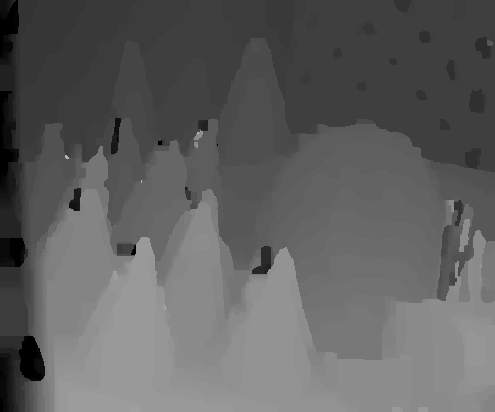
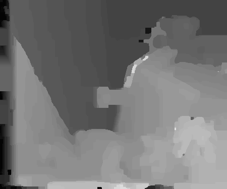
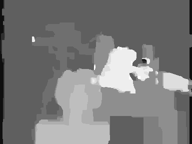
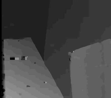
But speed was expected. The result that genuinely surprised us was about quality. Look at the actual disparity maps — flip between the cheap certified labeling and the full optimisation:

Interactive · flip between the cheap and the full result

Kovtun — certified, cheap Full optimisation Ground truth

Showing: Kovtun’s certified labeling

They are nearly indistinguishable. And when we measured error against ground truth, the cheap Kovtun labeling was, in the majority of cases, more accurate than the full α-expansion solution — even though α-expansion reaches a lower energy. That sounds paradoxical until you remember what energy is: a model of the world, not the world itself. Driving the energy to its absolute minimum optimises the model harder, and the model’s small biases harder along with it. The certified pixels are the ones the data was sure about in the first place — so the part we can prove is also the part that is most often right.

The practical reading is liberating: for a time-critical system — a robot, a camera, anything with a deadline — you can stop after the cheap phase and ship a labeling that is both fast and, on these benchmarks, often better. The expensive global optimum is optional.

Why a stereo paper sits in an AI portfolio

This work is older than the deep-learning era, and stereo depth is largely a learned problem now. I keep it here for what it shows about how I think, which has not dated. Three habits run through it and through everything I have built since. First, find the structure that makes a hard problem easy — the whole paper turns on noticing that a k-way labeling hides a binary search. Second, earn guarantees rather than hope for them: persistency is a proof, not a heuristic, and knowing which of your outputs are certified is exactly the kind of calibrated confidence modern ML systems are still scrambling to provide. Third, respect the gap between the objective and the goal — the surprise in this paper is a small, friendly version of the reward-hacking and over-optimisation problems that define a lot of frontier AI work today.

Faster algorithms, provable partial answers, and a healthy suspicion of the objective you are minimising: that is a toolkit, and it transfers. If your team is working on problems where those instincts would help, I would love to talk.